|
ARTICLES & HOW-TOS |
Spreadsheets for Modelling Calculations
Rich Brayshaw
Spreadsheets are used for organizing numerical data and are ideally suited to making multiple calculations from a few inputs. The spreadsheet used for this tutorial is provided by Open Office, and can be downloaded for free from www.openoffice.org The techniques demonstrated in this tutorial can be applied in any other spreadsheet, such as Excel but the specific commands may vary. Check your user’s manual if any problems occur.
A Simple Scale Calculator
Any of the cells can contain various numbers, text, images etc. and formulas. Start by making a simple spreadsheet to calculate various scales.
First, we need to input two numbers: the measurement and the scale. The cells we are going to input the data into can be labeled with text. We also want a cell in which the output will appear.
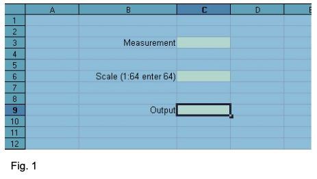
In Fig.1, text has been entered into cells B3, B6 and B9. It doesn’t matter which cells you use. Organize the spreadsheet to suit your needs. Column B has been made wider to accept a line of text that exceeds its width. Make columns wider by clicking on the dividing line between columns and dragging to the required width.
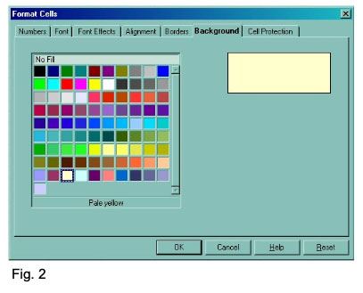
The cells that will contain the inputs and output have been given a background color. This is illustrated in Fig. 2.
- Highlight the cell or cells you wish to change. To select multiple cells, hold down the control key while you click.
- Right click inside one of them. Select ‘Format Cells’ from the context menu that appears.
- Select the ‘Background’ tab.
- Choose the desired background colour.
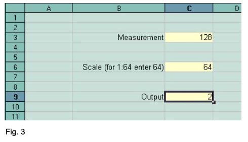
Now we will enter a formula into cell C9 to give us our results. We want to take a measurement and divided it by the scale to get the required scaled measurement. In this example, the Measurement entered into cell C3 needs to be divided by the Scale entered into cell C6. The result needs to appear in cell C9.
- Select C9
- Enter the formula: =C3/C6
The ‘=’ means a formula will be entered in this cell. The ‘/’ means divide. Don’t worry about the #VALUE! message that might appear in the cell. It just means a formula is waiting for data to be added in cells C3 and C6.
Let’s test the formula. Enter ‘128’ into cell C3 and ‘64’ into cell C6. The Output is '2'. (Fig. 3).
A More Advanced Scale Calculator
Let’s take the spreadsheet a stage further. This time we’re going to take a measurement in feet and convert it to millimeters and then scale it. Set up the spreadsheet as shown in Fig. 4 and enter the following formula into cell E5. =(C3*12+E3)*25.4
‘=’ means we’re entering a formula
‘(C3*12+E3)’ means we’re converting the feet entered in cell C3 to inches by multiplying by 12 and then adding the inches entered in cell E3.
25.4 is the conversion factor to convert from inches into millimeters.
Notice that when you select a cell that contains a formula, the formula also appears in the input line above the column letters. Formulas can also be entered here.
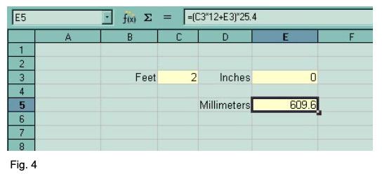
Now we can scale the measurement in millimeters using the method we used in the first example. Notice the formula for cell E9 in the input line. This spreadsheet shows us that 2 feet is equivalent to 9.53mm at 1:64 scale.
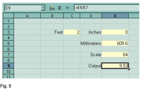
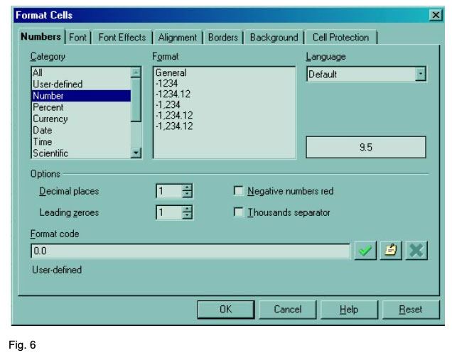
Let's do a bit of tidying up. It’s unlikely that you’ll need to measure to the nearest hundredth of a millimeter, so the final output can be formatted to display to the desired number of decimal places. Fig. 6 shows the dialogue box for formatting numbers. Note the other tabs for other ways in which the cells can be formatted.
- Right click the output cell and select ‘Format Cell’ from the context menu.
- Click on the ‘Numbers’ tab
- Change the number of ‘Decimal places’ to 1
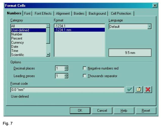
Next, we will label the units of the output figure to show millimeters. Still on the formatting menu we want to select ‘User-defined’ from the Category list, and enter “mm” to the ‘Format code’ (Fig. 7). Any text that is entered between inverted commas (“ ”) will appear after any data entered in the cell.
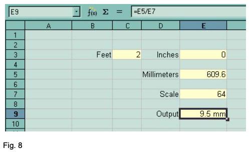
This is the re-formatted cell E9 in the spreadsheet. The result of the calculation is displayed to one decimal place and is labeled with millimeters (fig. 8)
Now we’re going to take what we’ve learned so far and apply it to making a spreadsheet to work out mast tapers.
Using the Spreadsheet to Work Out Mast Tapers
Depending on the vessel and period, masts and yards were tapered according to formulas. Steel’s The Elements and Practice of Rigging and Seamanship Vol. 1 has tables of data showing the measurements worked out for various diameters of mast. This reference work can be found online at https://maritime.org/doc/steel/index.htm
The length of mast determines its diameter at the partners (where the mast is at it greatest diameter as it passes through the upper deck). The diameter of the mast at the partners determines the diameters at the various quarters, the head and the heel.
From Steel The Elements and Practice of Rigging and Seamanship Vol. 1 p39
The diameters in proportion to the length, in the royal navy, are as follow: viz.
The main and foremasts of ships of 100 to 64 guns inclusive, are one inch in diameter at the partners to every yard in length. Ships of 50 to 32 guns inclusive, 9/10 of an inch to every yard in length. And ships of 28 guns and under, 7/8 a of an inch to every yard in the length.
The main-mast of brigs to be one inch to every yard in length, and the foremast 9/10 of the diameter of the main- mast.
The following table is from Steel The Elements and Practice of Rigging and Seamanship Vol. 1 p42
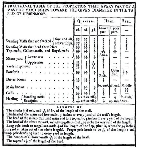
Knowing the diameter of the mast at the partners, we can get the spreadsheet to work out the various diameters throughout the length of the mast. Note that there are fore and aft, and athwartships dimensions for the heads, which were wider athwartships (6/7 of the diameter at the partners) than they were fore and aft (3/4 of the diameter at the partners).
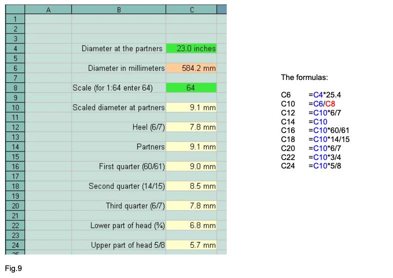
Lets get this information into a spreadsheet. I’ve set mine up as shown in Fig. 9. By now, you should be able to work out the formulas to enter into the relevant cells. I’ve listed them next to the example spreadsheet for the work-shy. I’ve also highlighted the cells that require input in green.
Next, consider that we need three masts. All of the cells can be copied to another part of the spreadsheet without worrying about the formulae we’ve entered. The cells named in the formulae are automatically updated to the new locations. We need to copy the table we’ve made twice, for the foremast and the mizzen. Simply highlight the areas to be copied (click and drag), copy (control C), click the top left cell of the area where they are to be pasted, and paste (control V).
We know the diameters of the masts at the partners from the data in Steel (p49), and these can be entered into the relevant green cells. Of course, Steel provides us with the various diameters of the masts too, but the spreadsheet automatically converts these to millimetres and at the required scale (Fig. 10)
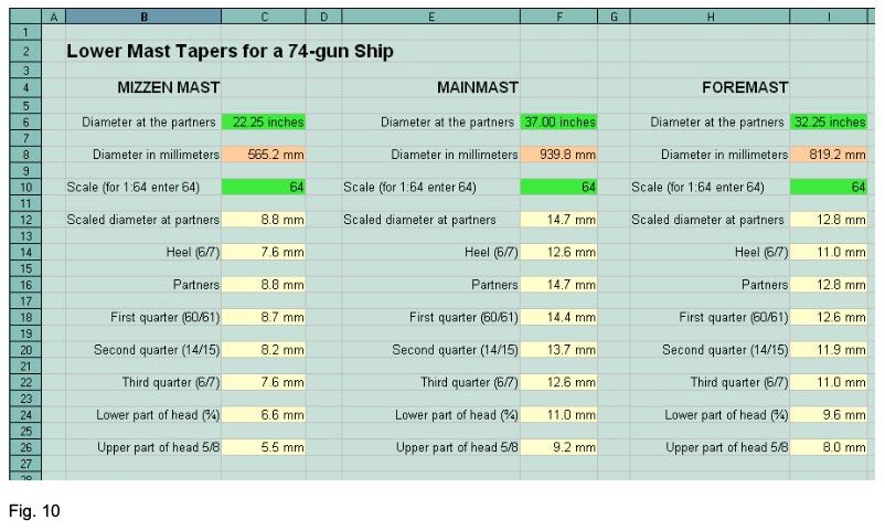
Some of the data in this spreadsheet are redundant – for example, the scale has been entered three times, and the diameter of the mast in millimetres before scaling isn’t a required measurement for the model. It can, however, be useful to include such results in the design of your spreadsheet as it makes it easier to troubleshoot. I also think it’s good practice not to have long formulas, for the same reason.
It’s possible, given the way mast and yard dimensions are calculated, to design a spreadsheet that will produce all the required mast and yard dimensions upon entering very few figures.
From Steel (p39) ...
The length of the lower deck and extreme breadth being added together, the half is the length of the main-mast.
If we know the length of the mainmast, then ...
Fore-mast, 8/9 of the main-mast. Mizen-mast, 6/7 of the main-mast.
If we know the mast lengths, then ....
Main-yard, 8/9 of the main-mast. Fore-yard, 7/8 of the main-yard. Etc, etc
So, if anyone is feeling inspired ...
|
© 2023 The Nautical Research Guild, Inc. Nautical Research Guild ® and the NRG logo are Registered Trademarks, and belong to the Nautical Research Guild (United States Patent and Trademark Office: No. 6,999,236 & No. 6,999,237, registered March 14, 2023)
|
![]()
© 2020 The Nautical Research Guild, Inc.
![]()